CAPM – Capital Asset Pricing Model

CAPM – Capital Asset Pricing Model

The CAPM is a staple of most every finance course that focuses on the valuation of equity investments. And though it may be a very good way to begin the process of teaching students how to effectively analyze securities there are a lot of assumptions that make it very difficult to use in a real world setting.

These assumptions are as follows –

• Investors hold a diversified portfolio
  • If you have a large enough portfolio or are focused entirely on ETF’s you may be able to get rid of the majority of the unsystematic risk within your portfolio, but for many people they are looking to analyze individual companies and project their returns.
• Single-period transaction horizon
  • If you are consistently rebalancing your portfolio this assumption isn’t that detrimental to the average portfolio, but if you are holding for longer than a single period the model falls apart.
• Investors can borrow and lend at the risk-free rate of return
  • Investors can easily lend at this rate, but it is unlikely they can borrow at this rate as they are not large institutions with access to those sorts of credit lines.
• Perfect capital markets
  • If you take a look at markets as a whole, including all traded financial instruments you may get an efficient market, but as an equity investor “the market” typically denotes the S&P 500 which is a much smaller representation of the general market.

So, already we can see that the CAPM may not be a good tool for investing into individual securities, but without testing we really can’t say that for certain.

Before we create the CAPM in Equities Lab we need the general formula to build from.

The Formula

E[r_i]=r_f+B_i(E(r_m)-r_f)

• E[r_i]= Asset return
• R_f= Risk free rate
• B_i= Beta for asset
• E(r_m) = Market return

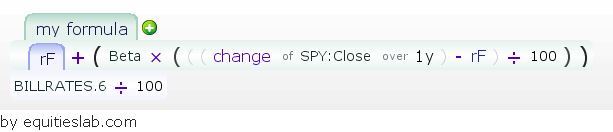
EquitiesLab CAPM Formula

First we create the CAPM formula using the most common period of 1 year as our single period assumptions.

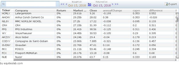
Using the basic screener for Basic Materials within the Equities Lab software we are presented with 201 matches. Since we don’t have data of the future, we can see how accurate the CAPM was over the past year when compared with the returns of each company.

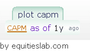
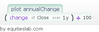
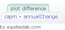
These three tabs just plot the CAPM, the previous year’s returns, and the difference between the two.

So, as you can see the CAPM isn’t really all that accurate when it comes to estimating real life returns of individual assets, but it was never supposed to. In the CAPM every asset is completely diversified and all unsystematic risk has been eliminated. Furthermore, all assets fall on the SML, or Security Market Line, which has a linear relationship between beta and return. In theory this is great, but in practice it doesn’t really fly. The CAPM Is still incredibly valuable when teaching students the basics of equity pricing, but it doesn’t have much of a place in our portfolios.